| time | status | idade | sexo | karno | tratamento | |
|---|---|---|---|---|---|---|
| Min. :0.002369 | Min. :0.0000 | Min. :33.00 | F:160 | Min. : 50.00 | 1: 83 | |
| 1st Qu.:0.196642 | 1st Qu.:1.0000 | 1st Qu.:54.00 | M:140 | 1st Qu.: 63.00 | 2: 93 | |
| Median :0.537423 | Median :1.0000 | Median :60.00 | NA | Median : 76.00 | 3:124 | |
| Mean :0.925945 | Mean :0.7733 | Mean :60.63 | NA | Mean : 76.04 | NA | |
| 3rd Qu.:1.353466 | 3rd Qu.:1.0000 | 3rd Qu.:68.00 | NA | 3rd Qu.: 90.00 | NA | |
| Max. :4.970028 | Max. :1.0000 | Max. :84.00 | NA | Max. :100.00 | NA |
Introduction
A randomized clinical trial was carried out to compare 3 different types of treatments used to treat patients diagnosed with lung cancer. The variables obtained after carrying out the study are:
- time: patient survival time, measured in years.
- status: variable indicating failure (1) or censorship (0).
- age: patient’s age, in years.
- sex: patient’s sex.
- karno: Karnofsky performance score, measured by the doctor.
- treatment: treatment received by the patient (three types of treatments: 1, 2 and 3).
Brief Descriptive Analysis of the Database
Let’s start by getting to know a little about our database.
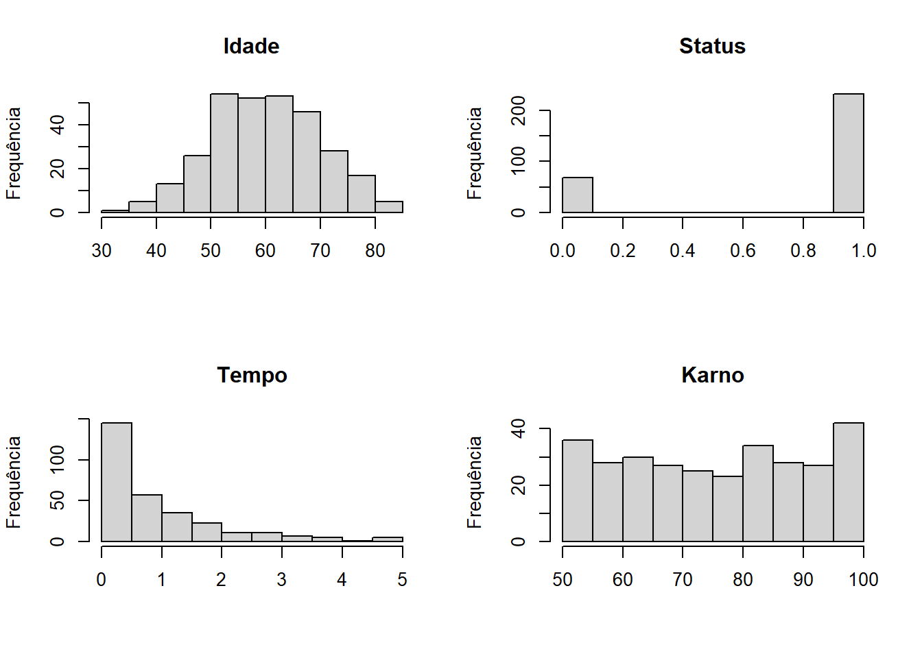
We can see some important things, we have an average time of 0.92 (years), but with a median of 0.53, which indicates an asymmetric distribution. We can also see that age and karno have more symmetrical distributions and that treatment group 3 is the largest among the 3 researched, among other things.
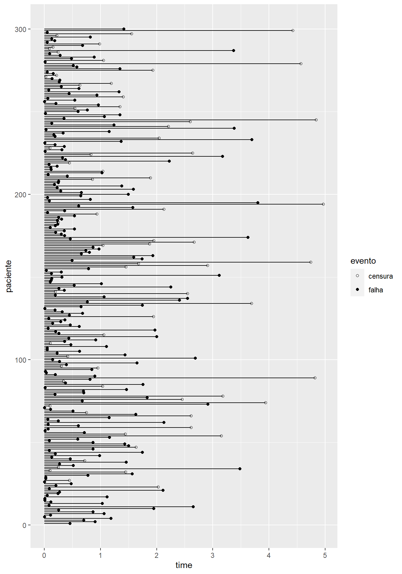
Additionally, see the failure and censorship graph below.
Lung Survival Analysis
Model Choice
Now let’s test the main survival analysis models seen during the Survival Analysis discipline. We will use as structures the Cox model as a non-parametric option and the Accelerate Failure Time, Proportional Hazards, Proportional Odds, Accelerated Hazard and Yang and Prentice models using the Exponential, Weibull, Log-Normal and Log-Logistic distributions as distribution possibilities.
It is worth noting that each adjustment was made stepwise in order to obtain the best model for that combination.
Now we will analyze which models achieved the best fit to the data. See Table.
| Model | AIC | Formula | Distribution |
|---|---|---|---|
| AFT | 457.9999 | Surv(time, status) ~ idade + sexo + tratamento | exponential |
| PH | 457.9999 | Surv(time, status) ~ idade + sexo + tratamento | exponential |
| PO | 447.8186 | Surv(time, status) ~ idade + tratamento | exponential |
| YP | 449.9697 | Surv(time, status) ~ idade + tratamento | exponential |
| AFT | 452.5137 | Surv(time, status) ~ idade + sexo + tratamento | weibull |
| PH | 452.5136 | Surv(time, status) ~ idade + sexo + tratamento | weibull |
| PO | 447.0453 | Surv(time, status) ~ idade + tratamento | weibull |
| YP | 451.6039 | Surv(time, status) ~ idade + tratamento | weibull |
| AFT | 462.7182 | Surv(time, status) ~ idade + tratamento | lognormal |
| PH | 461.6407 | Surv(time, status) ~ idade + tratamento | lognormal |
| PO | 473.8168 | Surv(time, status) ~ idade + tratamento | lognormal |
| YP | 461.8633 | Surv(time, status) ~ idade + tratamento | lognormal |
| AFT | 451.0738 | Surv(time, status) ~ idade + tratamento | loglogistic |
| PH | 452.6900 | Surv(time, status) ~ idade + sexo + tratamento | loglogistic |
| PO | 451.0738 | Surv(time, status) ~ idade + tratamento | loglogistic |
| YP | 453.3683 | Surv(time, status) ~ idade + tratamento | loglogistic |
The models that achieved the best fit, taking into account the lowest AIC, were the PO models with weibull and exponential distributions, respectively. Let’s test the possibility of using the most parsimonious model, that is, the exponential model. See the adjustments obtained below:
# A tibble: 5 × 6
  type        parameter   estimate      se  `2.5%` `97.5%`
  <chr>       <chr>          <dbl>   <dbl>   <dbl>   <dbl>
1 coefficient idade         0.0498 0.00953  0.0311  0.0685
2 coefficient tratamento2  -2.04   0.288   -2.61   -1.48
3 coefficient tratamento3  -0.889  0.252   -1.38   -0.396
4 baseline    alpha         1.13   0.0782   0.978   1.28
5 baseline    gamma         3.90   1.50     0.967   6.83
# A tibble: 4 × 6
type parameter estimate se `2.5%` `97.5%`
<chr> <chr> <dbl> <dbl> <dbl> <dbl>
1 coefficient idade 0.0380 0.00556 0.0271 0.0489
2 coefficient tratamento2 -1.97 0.281 -2.52 -1.42
3 coefficient tratamento3 -0.861 0.246 -1.34 -0.378
4 baseline lambda 0.369 0.108 0.157 0.580 As 1 is within the confidence interval for the alpha estimate in the model with a Weibull base distribution, we can use the exponential model for our analysis without losing much information. We will perform the likelihood ratio test to test whether the model can be simplified.
exponential(po) 1: Surv(time, status) ~ idade + tratamento
weibull(po) 2: Surv(time, status) ~ idade + tratamento
---
loglik LR df Pr(>Chi)
exponential(po) 1: -219.9093 2.7733 1 0.09585 .
weibull(po) 2: -218.5226 - - -
---
Signif. codes: 0 '***' 0.001 '**' 0.01 '*' 0.05 '.' 0.1 ' ' 1Since the p-value obtained was greater than the 5% significance level, we will reduce the PO model that uses the Weibull model as its base distribution to a PO model that uses exponential distribution as its base, since we did not reject the null hypothesis of the test .
Therefore, the model chosen to follow the analysis was a Proportional Odds model whose base chance is exponential distribution with \(\lambda = 0.368\).
Residuals Analysis
Now we will analyze the residuals generated by the chosen model.
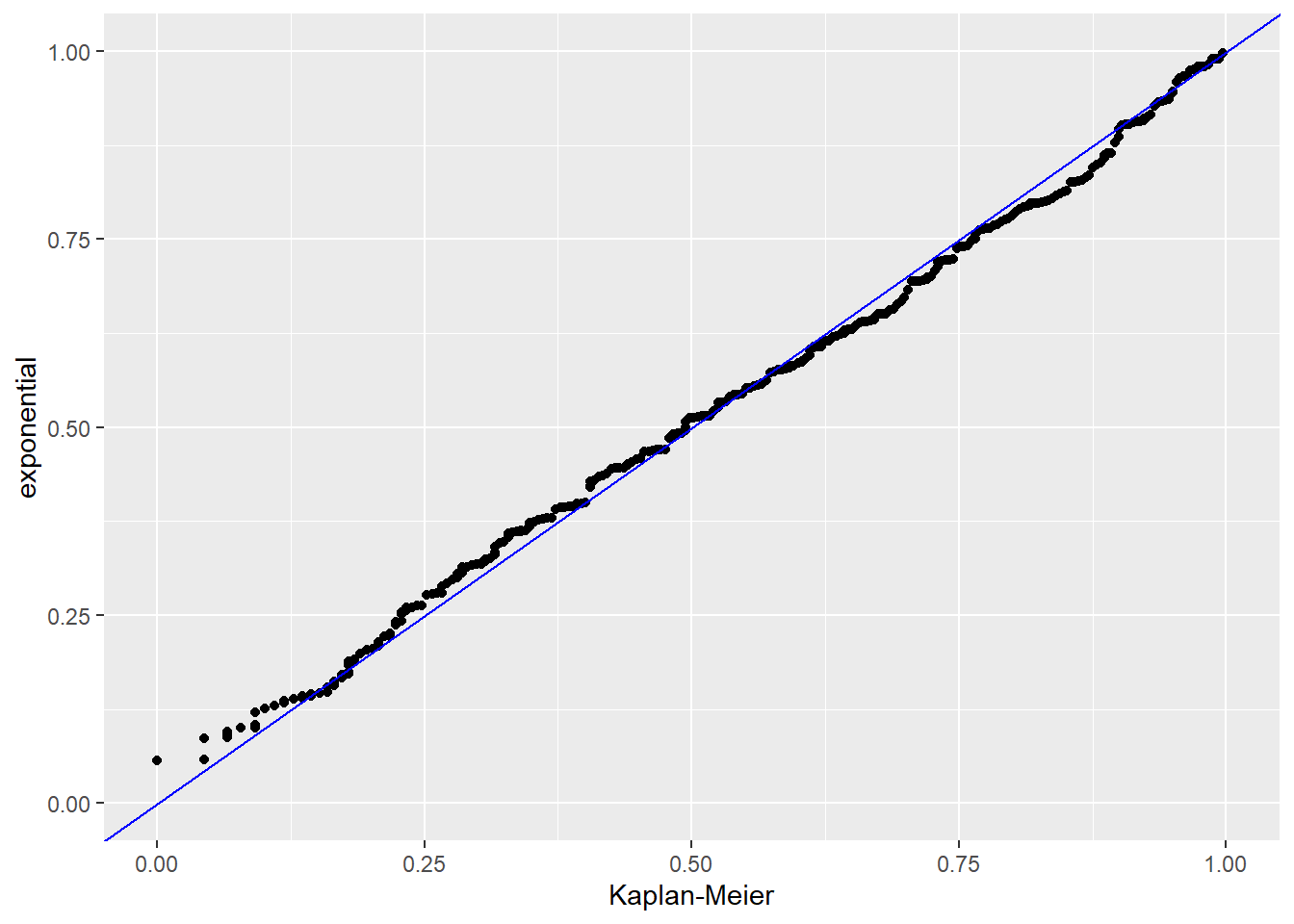
Analyzing the Cox Snell residual graph, it can be seen that the points fit well to the central line.
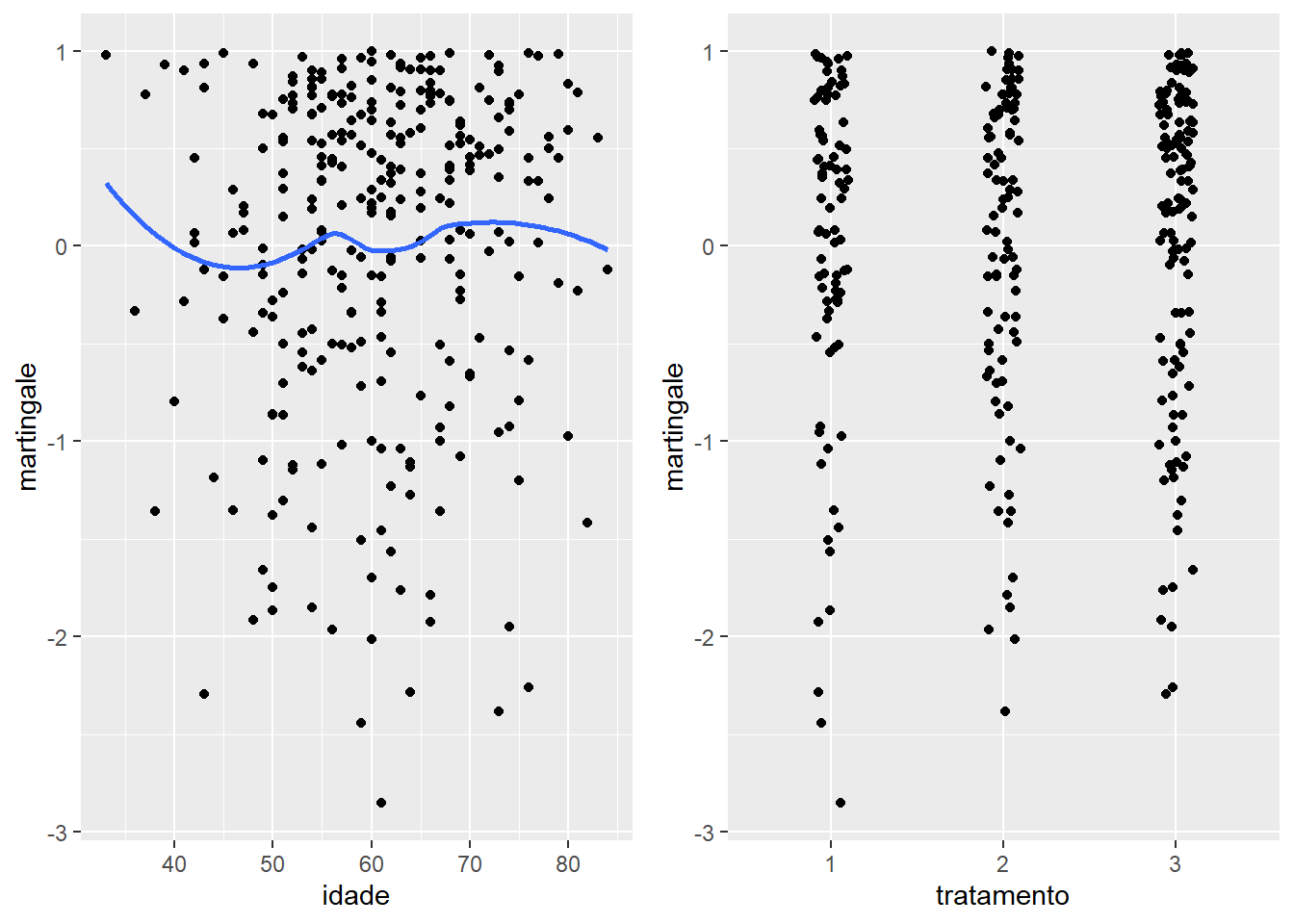
Analyzing the Martingale residual graph, it is noted that the points are randomly around zero.
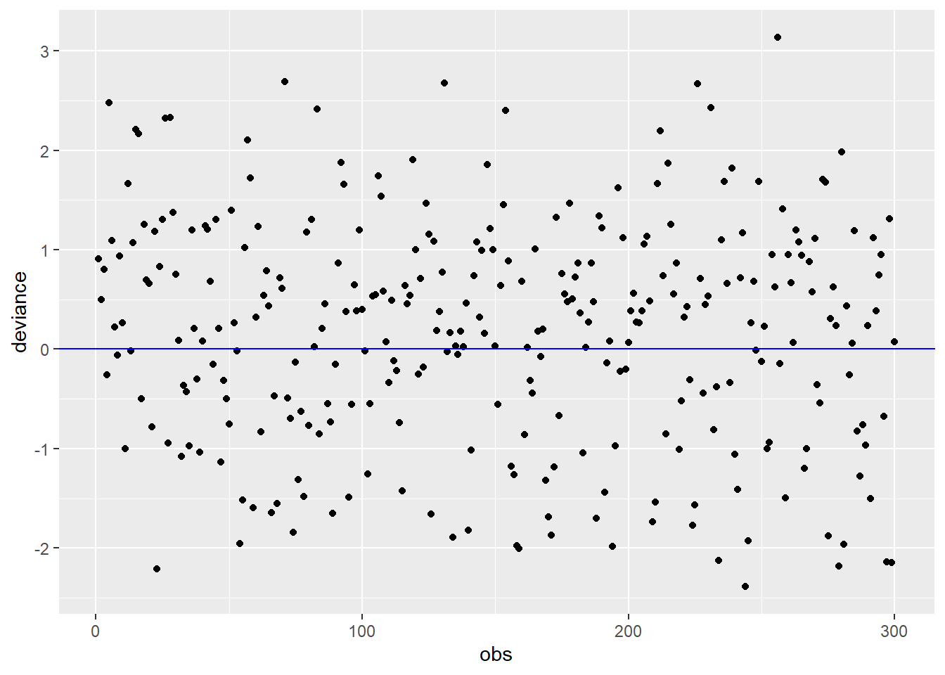
Analyzing the Deviance residual graph, it is noted that the points are randomly and symmetrical around zero.
Analysis of the results of the chosen model
Now that we have chosen a model and carried out its residual analysis, let’s analyze the results obtained. Recalling the model output:
# A tibble: 4 × 6
  type        parameter   estimate      se  `2.5%` `97.5%`
  <chr>       <chr>          <dbl>   <dbl>   <dbl>   <dbl>
1 coefficient idade         0.0380 0.00556  0.0271  0.0489
2 coefficient tratamento2  -1.97   0.281   -2.52   -1.42
3 coefficient tratamento3  -0.861  0.246   -1.34   -0.378
4 baseline lambda 0.369 0.108 0.157 0.580 The model is interpreted as follows:
The estimate of the \(\beta's\) obtained is exponentiated and affects the model’s base chance distribution. See the structure used by the Proportional Odds model:
\[ R(t|\Theta, \mathbf{x}) = R_{0}(t|\boldsymbol{\theta})\exp^{\mathbf{x} \boldsymbol{\beta}} \]
where \(R_{0}(t|\boldsymbol{\theta})\) is the base chance function that will have exponential distribution and \(\exp^{\mathbf{x} \boldsymbol{\beta}}\) are the covariates that will “disturb” the base chance function.
To measure this “disturbance” as a percentage, the following calculation is made:
\[ 100(e^{\beta}-1) \]
Therefore, we can make the following interpretations:
For the age variable:
- An increase of one unit in the age variable has an impact increase of 3.87% in the base chance function.
For the treatment variable:
In relation to treatment 1, the use of treatment 2 has an 86.1% lower impact on the base chance function.
In relation to treatment 1, the use of treatment 3 has a 57.73% lower impact on the base chance function.
Since the function’s output uses treatment 1 as its base, let’s look at Tukey’s multiple comparison to see the last remaining comparison, between treatment 2 and 3.
     General Linear Hypotheses

Multiple Comparisons of Means: Tukey Contrasts


Linear Hypotheses:
           Estimate
2 - 1 == 0   -1.973
3 - 1 == 0   -0.861
3 - 2 == 0 1.112- In relation to treatment 2, treatment 3 has a 204.04% greater impact on the base chance function.
Survival curves
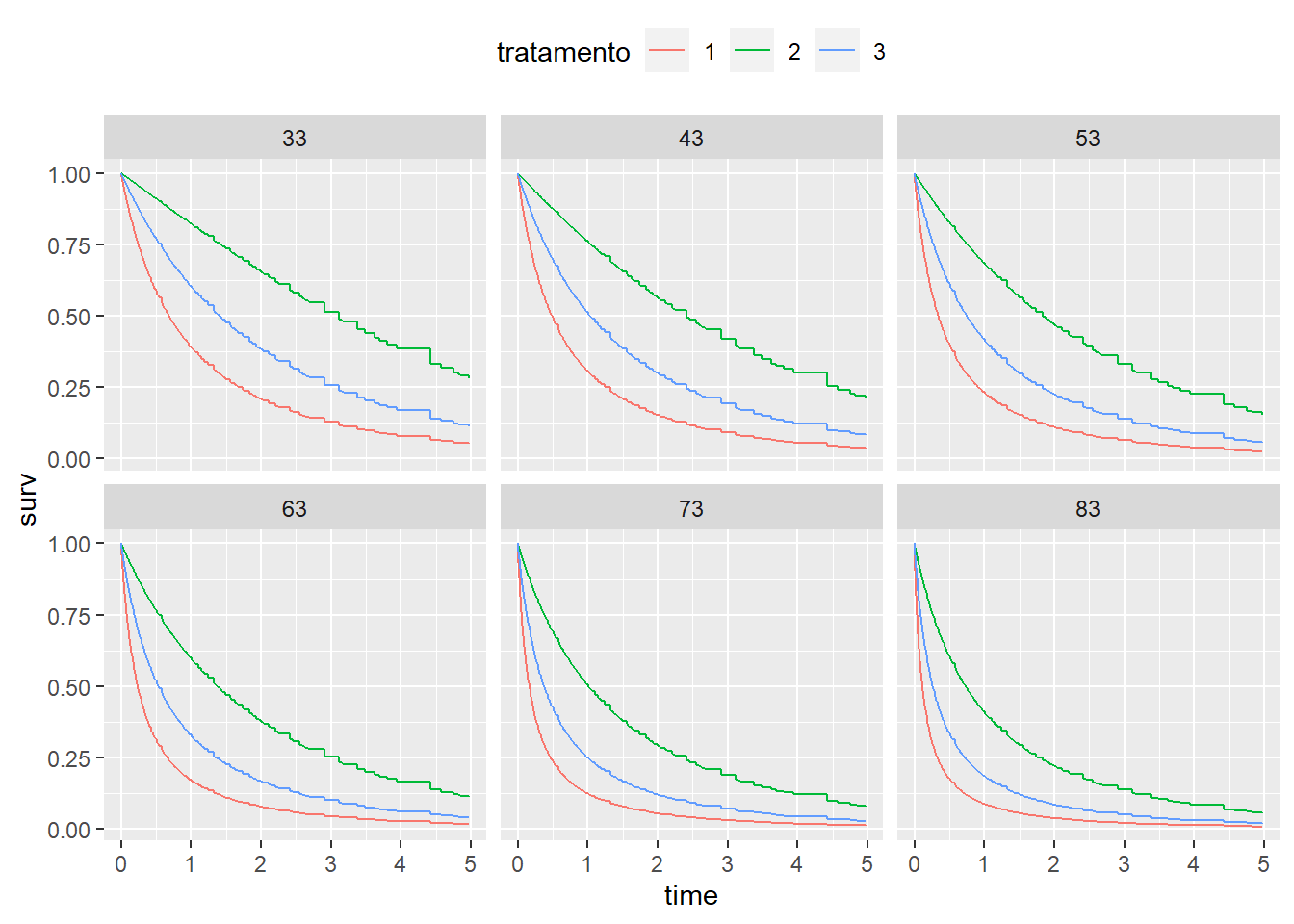
Let’s now test some possibilities for survival curve graphs for different ages in order to compare the groups.
Our minimum age in the lung database was 33 and the maximum was 84. Let’s look at the survival curves for different ages below.
Practical conclusions
Using Figure above as the main reference, we can note that at all ages, treatment 2 presented a survival curve superior to the other treatments. Furthermore, treatment 1 always presented the survival curve with the greatest decline at all ages. Consequently, treatment 3 obtained an intermediate survival curve compared to the others.
In section Analysis of the results of the chosen model it was highlighted that a one unit increase in the age variable has an impact increase of 3.87% on the base chance function. This fact was reinforced when the survival curves were made for different ages, since as age increased the curves declined more quickly.
Furthermore, when analyzing the \(\beta's\) of the treatment variable, treatments 2 and 3 had a smaller impact on the base chance function than treatment 1 and, when multiple comparisons were made to analyze the comparison between treatments 2 and 3 , treatment 3 had a 204.04% greater impact on the base chance function than treatment 2.
Therefore, the analysis carried out in the first paragraph in relation to Figure Survival curves for ages 33 to 83 by treatment was completely consistent with the analysis of \(\beta's\) and provided us with insights into the database of lung cancer cases.
References
R Core Team (2021). R: A language and environment for statistical computing. R Foundation for Statistical Computing, Vienna, Austria. URL https://www.R-project.org/.
survstan: Fitting Survival Regression Models via Stan. URL: https://cran.r-project.org/web/packages/survstan/index.html
Lawless (2002) ISBN:9780471372158;
Bennett (1982) doi:10.1002/sim.4780020223;
Chen and Wang(2000) doi:10.1080/01621459.2000.10474236;
Demarqui and Mayrink (2021) doi:10.1214/20-BJPS471.