| Ederson | V. Kompany | N. Otamendi | Danilo | İ. Gündoğan | Fernandinho | David Silva | L. Sané | F. Delph | Bernardo Silva | R. Sterling | |
|---|---|---|---|---|---|---|---|---|---|---|---|
| Ederson | 0 | 13 | 11 | 7 | 4 | 3 | 0 | 1 | 6 | 1 | 0 |
| V. Kompany | 13 | 0 | 29 | 18 | 12 | 12 | 6 | 1 | 10 | 1 | 5 |
| N. Otamendi | 11 | 29 | 1 | 2 | 13 | 24 | 20 | 9 | 40 | 0 | 9 |
| Danilo | 7 | 18 | 2 | 2 | 8 | 16 | 4 | 2 | 5 | 11 | 7 |
| İ. Gündoğan | 4 | 12 | 13 | 8 | 0 | 8 | 8 | 2 | 5 | 6 | 2 |
| Fernandinho | 3 | 12 | 24 | 16 | 8 | 0 | 32 | 11 | 23 | 7 | 5 |
| David Silva | 0 | 6 | 20 | 4 | 8 | 32 | 0 | 12 | 20 | 4 | 2 |
| L. Sané | 1 | 1 | 9 | 2 | 2 | 11 | 12 | 1 | 20 | 1 | 0 |
| F. Delph | 6 | 10 | 40 | 5 | 5 | 23 | 20 | 20 | 2 | 0 | 2 |
| Bernardo Silva | 1 | 1 | 0 | 11 | 6 | 7 | 4 | 1 | 0 | 0 | 4 |
| R. Sterling | 0 | 5 | 9 | 7 | 2 | 5 | 2 | 0 | 2 | 4 | 0 |
Introduction
Football is one of the most practiced and watched sports in the modern world, its tactical and technological evolution has been extensively documented over the years and data collection together with statistical analysis has become a powerful and increasingly necessary weapon for be successful on the pitch of the world’s biggest stadiums. The different tactics implemented can be attributed to how the 11 players on each team interact with each other, creating complex structures of relationships and positioning on the field. In this study, we intend to use the knowledge obtained from graph networks to gain insights into one of the biggest upsets in the Premier League.
Goal
Analyze and visualize the efficiency of passing networks between Manchester United and Manchester City players during the 17/18 Premier League season, using graphs. Identify connectivity patterns, key players in the distribution of passes and evaluate how these passing dynamics influenced the teams’ overall performance.
Database
The data for this work were extracted from the Kaggle platform, at the following link: https://www.kaggle.com/datasets/aleespinosa/soccer-match-event-dataset. This database brings together information on all actions in a football game, that is, we have the action (pass, kick, foul, etc.), which player is responsible for it, in which part of the field it occurred and at which point in the game it was made. The database contains all matches from the 17/18 season from five national leagues (La Liga, Serie A, Bundesliga, Premier League, Ligue 1), as well as the 2016 Euro Cup and the 2018 World Cup. For this work, we will use data of just one play from the match between Manchester United vs. Manchester City for the 17/18 Premier League season, which ended with a score of 3 x 2 for Manchester United. To do this, we need to load the following tables from the database: ‘features.csv’, ‘players.csv’ and ‘teams.csv’.
The tables contain: - features.csv: Data on each action during the Premier League 17/18 matches, for example: type of action, moment of the game that occurred, positions, etc.
players.csv: General player data, for example: name, full name, age, etc.
teams.csv: Data from all teams that participated in one of the five national leagues contained in the database and the teams that participated in the 2016 Europe or the 2018 World Cup.
Only interaction actions between two teammates on the same team that were successfully carried out were filtered. In other words, a kick, foul suffered or even a wrong pass, for example, did not enter our analysis, only: passes, throw-ins, crosses from set pieces (fouls and corners), passes from set pieces, goal kicks and “kicks” . Remembering that, only if carried out successfully.
Study and Analysis
The analysis was carried out by separating the two teams and studying the way in which the players on the team interacted during the match.
Manchester City
- Adjacency matrix:
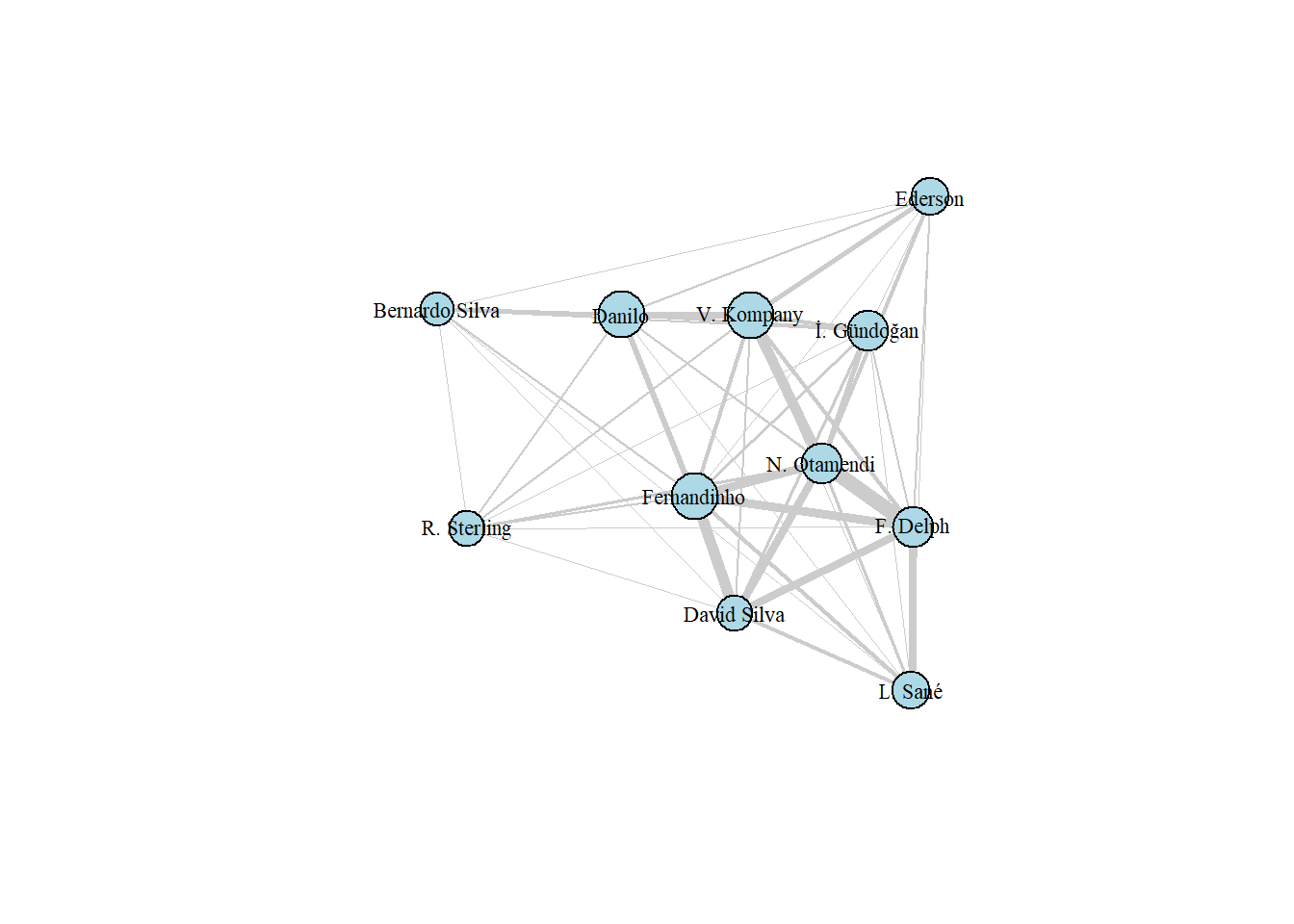
The Manchester City team graph containing only the starting players shows us some very interesting characteristics of the match.
Firstly, we can see from the thickness of the edges that the City team used players on the left side of the field a lot (left in relation to the team’s attacking direction), so Fernandinho, Delph, David Silva and Otamendi formed a strong concentration of interactions with each other.
Secondly, due to the size of the vertices, we can see the greater centrality of the defensive and midfield players, especially for Fernandinho who was the player with the greatest centrality, this is mainly due to the well-centralized position on the field and the function of interact with both defensive and attacking players, often having to act as a link between these two sectors of the field.
Thirdly, through the graph, it is clear how in this game City’s center forward isolated himself from the rest of the team, Bernardo Silva was the team’s starting center forward and in the graph we see low centrality and little thickness of the edges leaving his apex, which indicates that the player interacted little and with a small number of teammates in relation to the others. Next, we will present a descriptive analysis of this graph.
Descriptive analysis of the graph
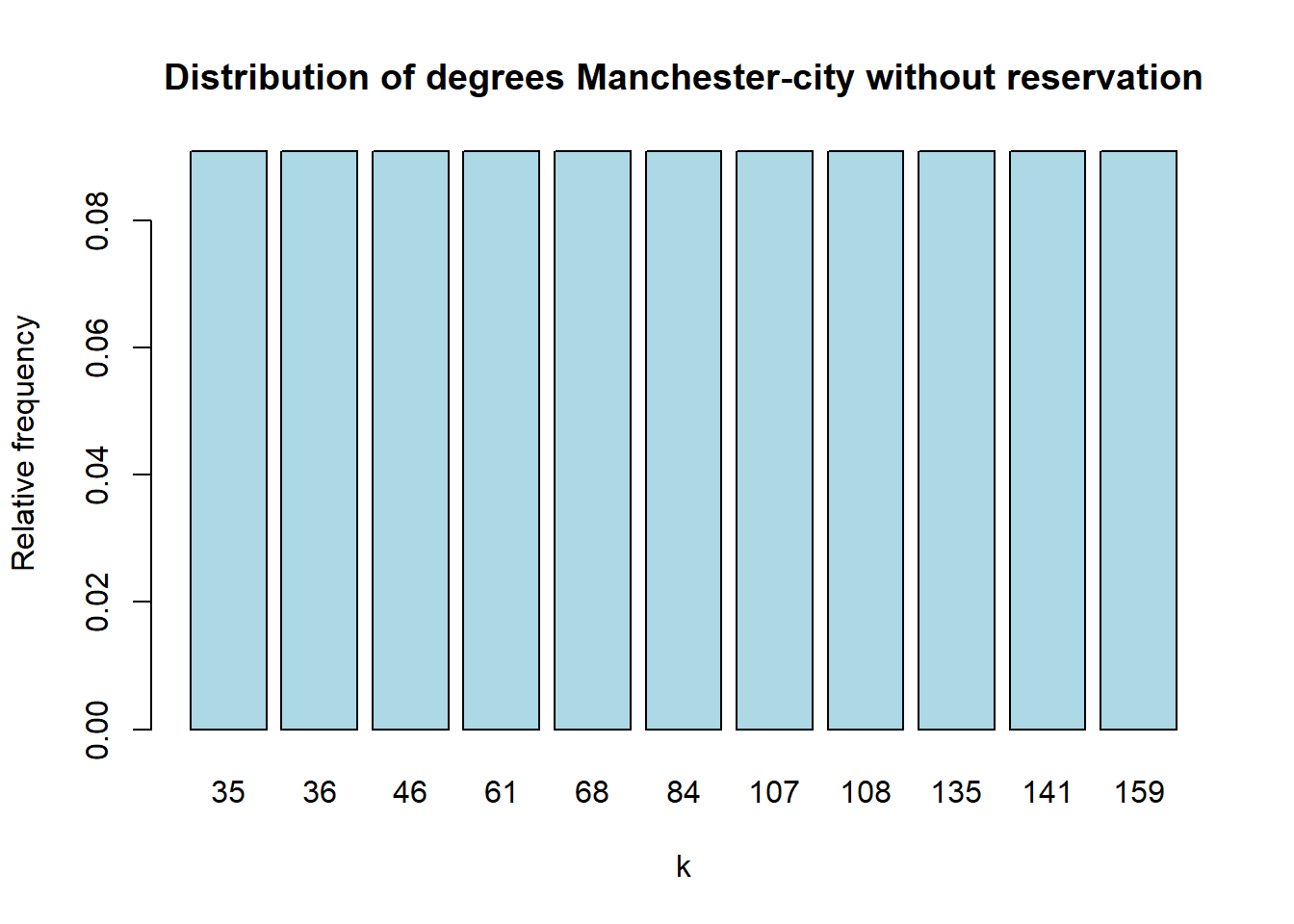
- DEGREE
The most basic measure of a graph is degree, the number of adjacent edges connected to each node. It is often considered a measure of direct influence. In networks related to the Manchester city team, it will be the number of players with which each player is interacting.
| Number of connections | |
|---|---|
| N. Otamendi | 159 |
| Fernandinho | 141 |
| F. Delph | 135 |
| David Silva | 108 |
| V. Kompany | 107 |
| Danilo | 84 |
| İ. Gündoğan | 68 |
| L. Sané | 61 |
| Ederson | 46 |
| R. Sterling | 36 |
| Bernardo Silva | 35 |
- CLOSENESS
Proximity measures how many steps it takes to access all other nodes from a given node. It is a measure of how long a player’s action takes to reach another player. Higher values mean less centrality.
| Number of connections | |
|---|---|
| V. Kompany | 0.10 |
| Danilo | 0.10 |
| İ. Gündoğan | 0.10 |
| Fernandinho | 0.10 |
| N. Otamendi | 0.09 |
| David Silva | 0.09 |
| L. Sané | 0.09 |
| F. Delph | 0.09 |
| Ederson | 0.08 |
| Bernardo Silva | 0.08 |
| R. Sterling | 0.08 |
- BETWEENNESS
The “Betweenness” measure is approximately the number of “shortest paths” between nodes that pass through some particular node.
| Number of connections | |
|---|---|
| Fernandinho | 1.29 |
| N. Otamendi | 1.12 |
| David Silva | 0.51 |
| V. Kompany | 0.51 |
| Danilo | 0.50 |
| F. Delph | 0.43 |
| İ. Gündoğan | 0.36 |
| R. Sterling | 0.10 |
| L. Sané | 0.10 |
| Ederson | 0.04 |
| Bernardo Silva | 0.04 |
Clustering the graph
In order to group players automatically, we use clustering with the cluster_walktrap function. This function tries to find densely connected subgraphs also called communities in a graph through random walks. The idea is that short random walks tend to stay in the same community.
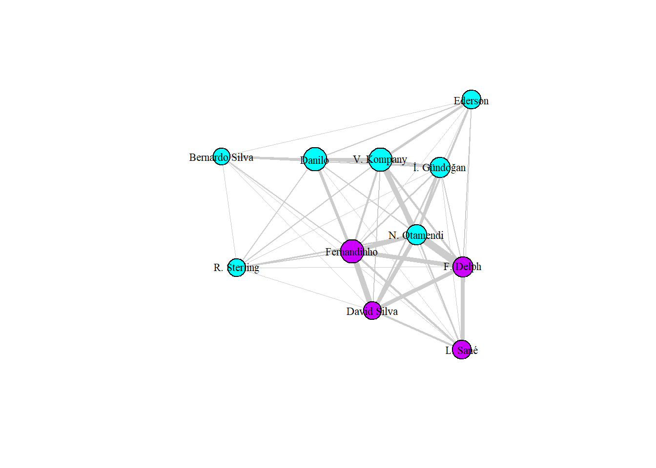
Since we used the tkplot function from the igraph package to adjust the players’ position, it was not possible to plot the graph generated by the cluster_walktrap function. Therefore, we obtained the colors given for each of the vertices as a result to differentiate in the final plot of the graph.
We can note that, for the clustered graph of Manchester City’s passing network, the method used divided the network into two clusters, one of them with players on the left side of the field, which we can see had high interaction with each other due to the thickness of the vertices. , in addition to another cluster that grouped the remaining players.
Manchester United
- Adjacency matrix:
| J. Lingard | N. Matić | A. Valencia | David de Gea | A. Young | C. Smalling | E. Bailly | Ander Herrera | P. Pogba | A. Sánchez | R. Lukaku | |
|---|---|---|---|---|---|---|---|---|---|---|---|
| J. Lingard | 1 | 9 | 9 | 3 | 5 | 0 | 0 | 7 | 2 | 2 | 1 |
| N. Matić | 9 | 1 | 13 | 4 | 7 | 5 | 8 | 15 | 10 | 3 | 2 |
| A. Valencia | 9 | 13 | 3 | 2 | 2 | 0 | 8 | 20 | 7 | 2 | 2 |
| David de Gea | 3 | 4 | 2 | 1 | 2 | 7 | 3 | 4 | 2 | 1 | 2 |
| A. Young | 5 | 7 | 2 | 2 | 3 | 8 | 3 | 4 | 7 | 9 | 1 |
| C. Smalling | 0 | 5 | 0 | 7 | 8 | 0 | 3 | 2 | 4 | 0 | 0 |
| E. Bailly | 0 | 8 | 8 | 3 | 3 | 3 | 0 | 5 | 1 | 2 | 1 |
| Ander Herrera | 7 | 15 | 20 | 4 | 4 | 2 | 5 | 2 | 9 | 1 | 4 |
| P. Pogba | 2 | 10 | 7 | 2 | 7 | 4 | 1 | 9 | 0 | 7 | 1 |
| A. Sánchez | 2 | 3 | 2 | 1 | 9 | 0 | 2 | 1 | 7 | 0 | 5 |
| R. Lukaku | 1 | 2 | 2 | 2 | 1 | 0 | 1 | 4 | 1 | 5 | 0 |
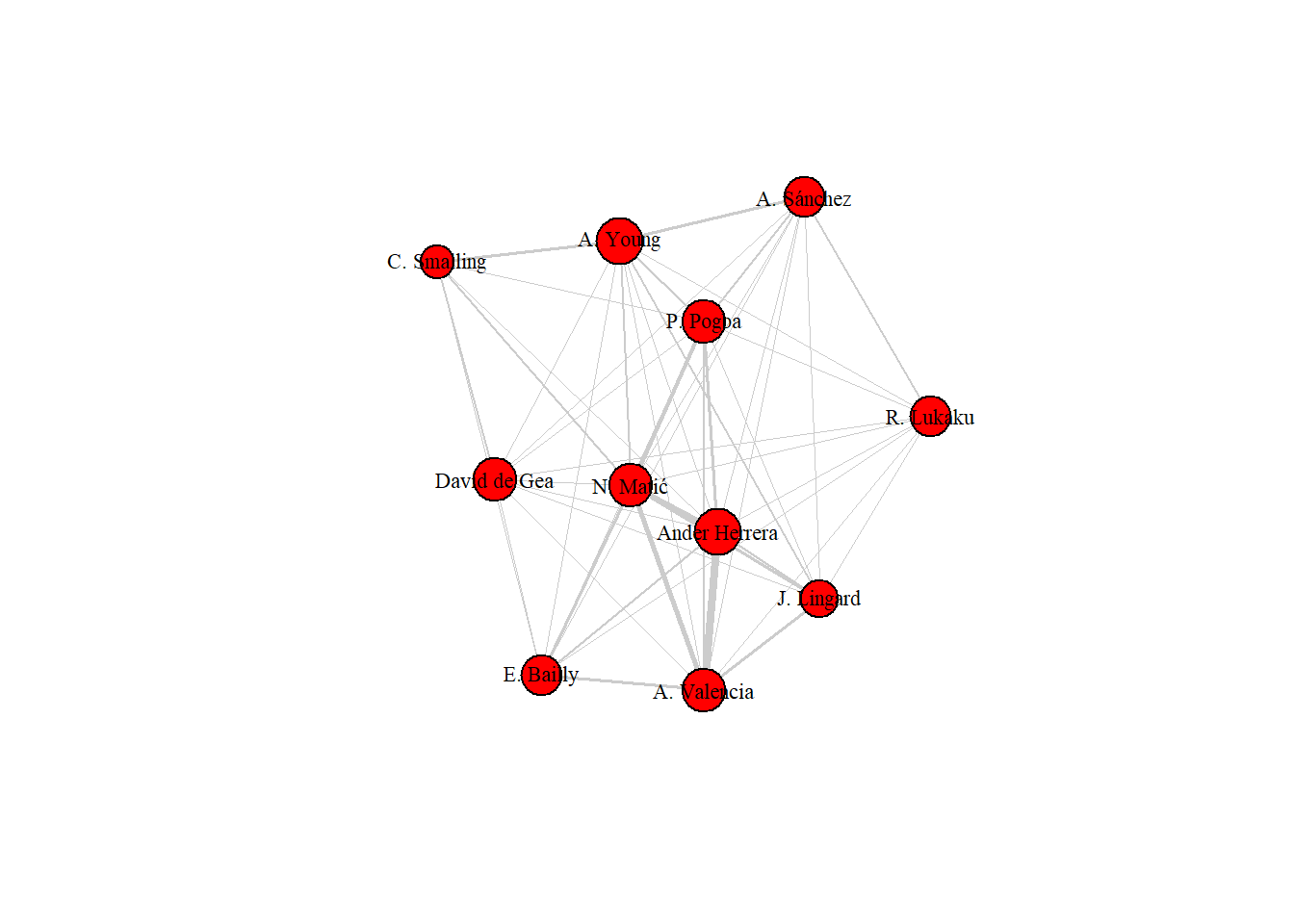
From the match graph of Manchester United’s starting players, we can understand some very interesting characteristics of the match.
Firstly, in relation to the thickness of the edges, in a “contrary” way (United’s Right = City’s Left) to City, United’s right side is the one with the thickest edges, indicating that there was greater passing interaction in this field region. Furthermore, looking at the size of the vertex, we notice that one of the players with the highest centrality is also in this region, Ander Herrera, midfielder.
Furthermore, through the graph, it is clear how in this game defender Smalling was not very involved in passing, given that he has low centrality and few connections with his teammates.
Descriptive analysis of the graph
The most basic measure of a graph is degree, the number of adjacent edges connected to each node. It is often considered a measure of direct influence. In networks related to the Manchester city team, it will be the number of players with which each player is interacting.
- DEGREE
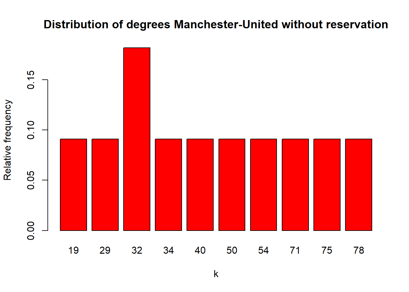
| Number of connections | |
|---|---|
| N. Matić | 78 |
| Ander Herrera | 75 |
| A. Valencia | 71 |
| A. Young | 54 |
| P. Pogba | 50 |
| J. Lingard | 40 |
| E. Bailly | 34 |
| David de Gea | 32 |
| A. Sánchez | 32 |
| C. Smalling | 29 |
| R. Lukaku | 19 |
- CLOSENESS
Proximity measures how many steps it takes to access all other nodes from a given node. It is a measure of how long a player’s action takes to reach another player. Higher values mean less centrality.
| Number of connections | |
|---|---|
| N. Matić | 0.10 |
| David de Gea | 0.10 |
| A. Young | 0.10 |
| Ander Herrera | 0.10 |
| P. Pogba | 0.10 |
| A. Valencia | 0.09 |
| E. Bailly | 0.09 |
| A. Sánchez | 0.09 |
| R. Lukaku | 0.09 |
| J. Lingard | 0.08 |
| C. Smalling | 0.07 |
- BETWEENNESS
The “Betweenness” measure is approximately the number of “shortest paths” between nodes that pass through some particular node.
| Number of connections | |
|---|---|
| N. Matić | 1.37 |
| A. Young | 1.19 |
| Ander Herrera | 0.68 |
| David de Gea | 0.63 |
| P. Pogba | 0.52 |
| A. Valencia | 0.34 |
| E. Bailly | 0.24 |
| A. Sánchez | 0.02 |
| R. Lukaku | 0.00 |
| J. Lingard | 0.00 |
| C. Smalling | 0.00 |
Clustering the graph
In order to group players automatically, we use clustering with the cluster_walktrap function. This function tries to find densely connected subgraphs also called communities in a graph through random walks. The idea is that short random walks tend to stay in the same community.
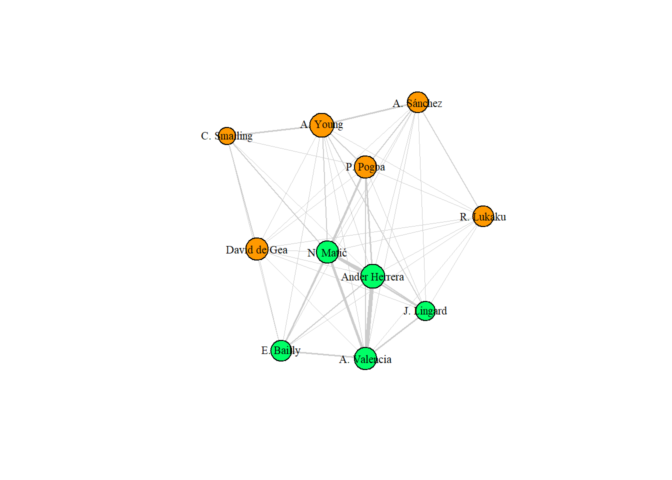
Since we used the tkplot function from the igraph package to adjust the players’ position, it was not possible to plot the graph generated by the cluster_walktrap function. Therefore, we obtained the colors given for each of the vertices as a result to differentiate in the final plot of the graph.
We can note that, for the clustered graph of Manchester United’s passing network, the method used divided the network into two clusters, one of them with players on the right side of the field, which we can see had greater interaction with each other due to the thickness of the vertices, in addition to another cluster that grouped the remaining players.
Conclusion
From the game statistics, we saw that City had 65% possession of the ball, making 596 passes compared to United’s 318. This greater participation in the game is evident when we look at the grade, with City players having much higher numbers than United players, for example, the player in City’s graph with the highest grade, as we saw in the table, was Otamendi (159 ) who had a grade greater than twice that of Matić, who was the player in the United graph with the highest grade (78).
Furthermore, as we saw in the graphs, the greater number of interactions on the left side of City’s formation and on the right side of United’s formation is noticeable. This indicates that the game was mostly concentrated in this sector of the field. However, even though Manchester City played a greater volume of games, they still left without winning the match.
In this way, this study can contribute to previous studies of team behaviors in different matches, aiming to understand the opposing team in order to obtain advantages in games.
References
Database: https://www.kaggle.com/datasets/aleespinosa/soccer-match-event-dataset
Passing Network of Football: https://rpubs.com/ihatestudying/passing-network-
Pascal Pons, Matthieu Latapy: Computing communities in large networks using random walks, https://arxiv.org/abs/physics/0512106
Freeman, L. C. (1979). Centrality in Social Networks I: Conceptual Clarification. Social Networks 1, 215–239.
Wasserman, S., and Faust, K. (1994). Social Network Analysis: Methods and Applications. CambridgeUniversity Press.