Introduction
The insurance market is the sector of the economy responsible for managing policy negotiations, protecting individuals, companies and beneficiaries from unforeseen financial losses. It is made up of some types of companies such as insurance companies, brokers, insurtechs, among others. Insurance is a contract that determines that one of the parties — called the insurer — undertakes, upon receipt of a payment — the premium —, to indemnify the other party — called the insured — in relation to losses provided for in the agreement. Let’s look at some important definitions used in this marke:
Premiums: The premium is the amount you pay to be entitled to the insurance coverage you have contracted. To be entitled to compensation, it is necessary to pay a specific amount, defined at the time of contracting. This payment is the prize. The amount of the insurance premium depends on some factors. Some of them are the type of insurance, the coverage offered by the policy and the risk profile of the insured.
Claim: In the insurance market, a claim refers to any event in which the insured property suffers an accident or material damage. It represents the materialization of risk, causing financial losses for the insurer. Having a claim means that a situation or damage covered by your insurance occurred. As such, you must take action so that your insurer can begin the entire process of repairing the damage or providing the compensation due.
Goal
The objective of this study is to create a statistical model that can estimate the claim (ocurred claim) of the 775 insurance sector in Brazil based on information from previous dates.
Sector 775 is known as Guarantee Insurance for the Public Sector. This insurance contract guarantees the faithful fulfillment of the obligations assumed by the policyholder towards the insured, in accordance with the terms of the policy and up to the value of the guarantee established therein, and in accordance with the modality(s) and/or coverage(s) additional(s) expressly contracted, due to participation in bidding, in a main contract pertinent to works, services, including advertising, purchases, concessions and permissions within the scope of the Powers of the Union, States, the Federal District and the Municipalities.
Data Base
The database used is from the SUSEP Statistics System (Private Insurance Superintendence). SUSEP is a federal agency linked to the Ministry of Economy in Brazil responsible for controlling and supervising the insurance, open private pension, capitalization and reinsurance markets.
The selected operation was Premiums and Claims grouped by sector, from January 2022 to November 2023, in order to analyze the premiums and claims of sector 775 - Guarantee for the Public Sector.
Dataset can be accessed at https://www2.susep.gov.br/menuestatistica/SES/principal.aspx.
Results
In this topic we will see a little about the behavior of our variable of interest: “Claim”. We will analyze how it behaves in relation to the other variables that will be used to estimate our model and, in addition, we will see the development of the model.
Descriptive Analysis of each variable
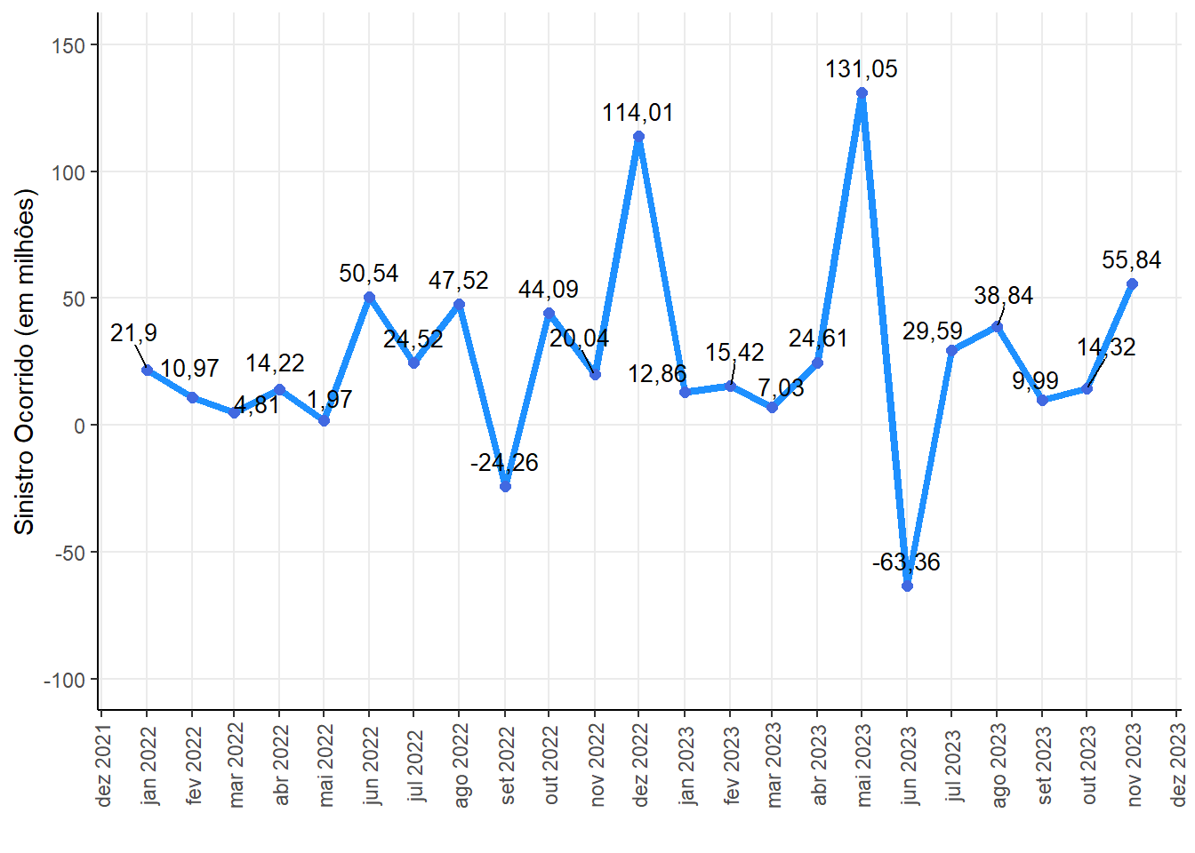
Historical series of the claim ocurred for the sector 775 - Insured Guarantee - Public Sector
An accident occurs refers to the occurrence of an event that causes damage or damage to an insured asset. For an event to be considered a claim, coverage for the event that occurred must have been contracted and be present in the policy during its validity.
Therefore, having a claim means that a situation or damage covered by your insurance occurred. As such, you must take action so that your insurer can begin the entire process of repairing the damage or compensating you.
Ocurred Claim (in million)
|
||||
|---|---|---|---|---|
| Min. | Median | Mean | Max. | Std Dev |
| -63,36 | 20,04 | 26,37 | 131,05 | 39,45 |
Historical series of the direct premium for the sector 775 - Insured Guarantee - Public Sector
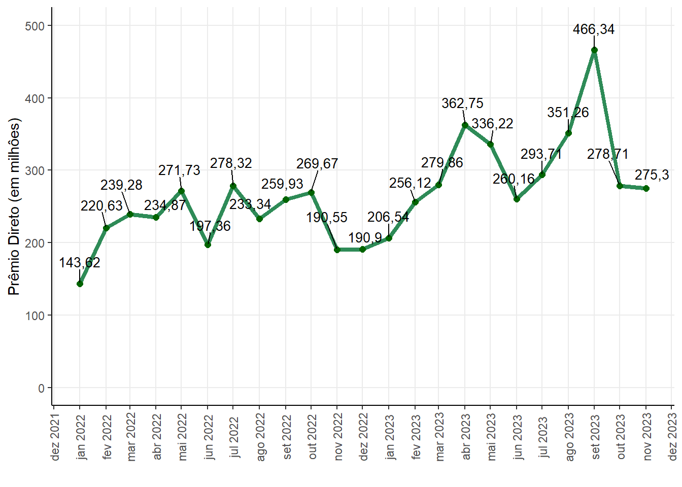
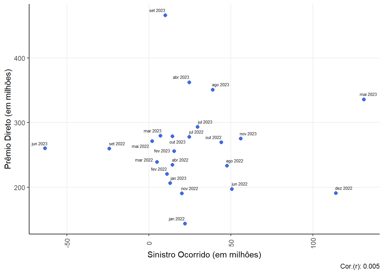
We can notice that since the beginning of 2022 the value of the direct premium for the 775 sector has increased and decreased at times. Its highest value was 466,34 million in September 2023, which has been increasing since June of that same year.
Direct Premium (in million)
|
||||
|---|---|---|---|---|
| Min. | Median | Mean | Max. | Std Dev |
| 143,62 | 260,16 | 265,09 | 466,34 | 68,3 |
Historical series of the earned premium for the sector 775 - Insured Guarantee - Public Sector
Earned premium refers to when policyholders pay premiums in advance, insurers do not immediately consider premiums paid for an insurance contract as earned. When the prize is paid, it is considered an unearned prize – not profit. This is because the insurer still has an obligation to fulfill. The insurance company can change the premium status from unearned to earned only when the entire premium is considered profit.
The main difference between earned premium and direct premium is that earned premium is the premium used during the period when the insurance policy was in force and insurance companies can record it as income after the premium coverage period ends. While the direct premium is the amount paid by the customer to the insurer in exchange for transferring the risk
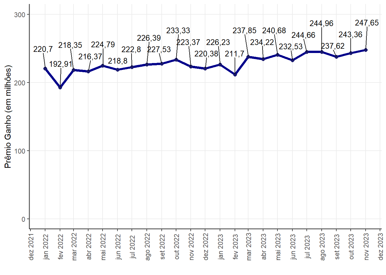
Regarding the earned premium from the Public Guarantee insurance sector, we can note that only on one date, since the beginning of 2022, this value was less than 200 million (February 2022). The peak point was in November 2023, where a prize win of 247,65 million was recorded.
Earned Premium (in million)
|
||||
|---|---|---|---|---|
| Min. | Median | Mean | Max. | Std Dev |
| 192,91 | 226,39 | 228,14 | 247,65 | 12,81 |
Historical series of the reinsurance expense for the sector 775 - Insured Guarantee - Public Sector
Reinsurance is a practice that allows insurers to transfer part of the risks they assume to other companies, called reinsurers. This is done to protect the assets and operational results of insurance companies, increase their retention capacity, offer protection against risks caused by catastrophes and stabilize the loss ratio.
Reinsurance expense refers to the total value of premiums allocated to reinsurers, in addition to their participation in all claim payments. In other words, it is the cost that the insurer has to transfer part of the risks it has assumed to the reinsurer. This amount is paid as a reinsurance premium by the insurer (or cedant) to the reinsurer.
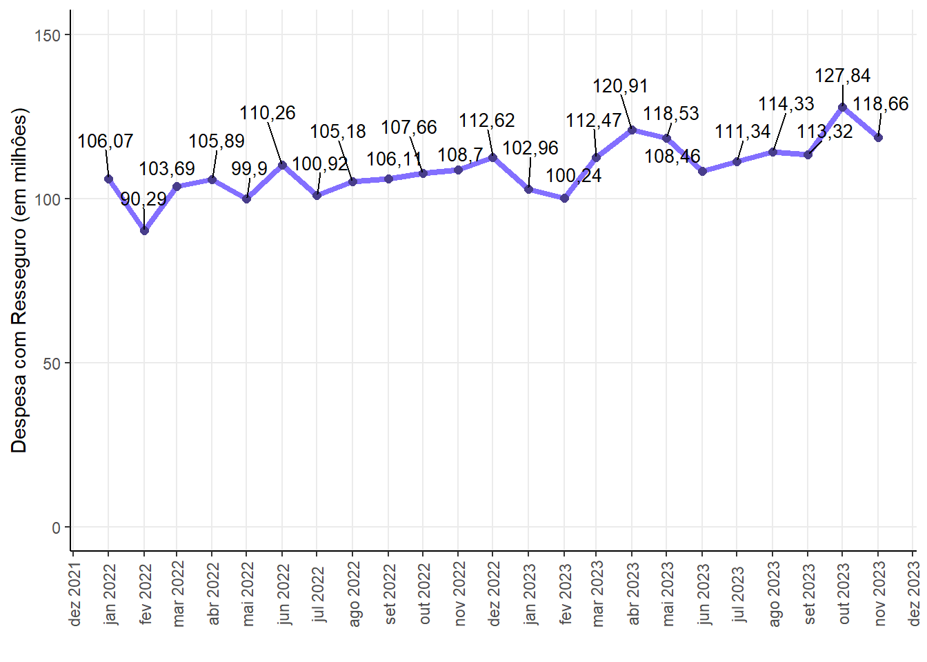
Regarding reinsurance expenditure, the lowest expenditure on the 775 insurance sector was in February 2022. Furthermore, the highest expenditure was recorded in October 2023, with a value of 127,84 million.
Reinsurance Expense (in million)
|
||||
|---|---|---|---|---|
| Min. | Median | Mean | Max. | Std Dev |
| 90,29 | 108,46 | 108,97 | 127,84 | 8,1 |
Historical series of the reinsurance income for the sector 775 - Insured Guarantee - Public Sector
Reinsurance income is the premium that the insurer (or cedant) receives from the reinsurer in exchange for transferring part of the risks that the insurer has assumed. This premium is paid by the reinsurer to the insurer and is considered income for the insurer.
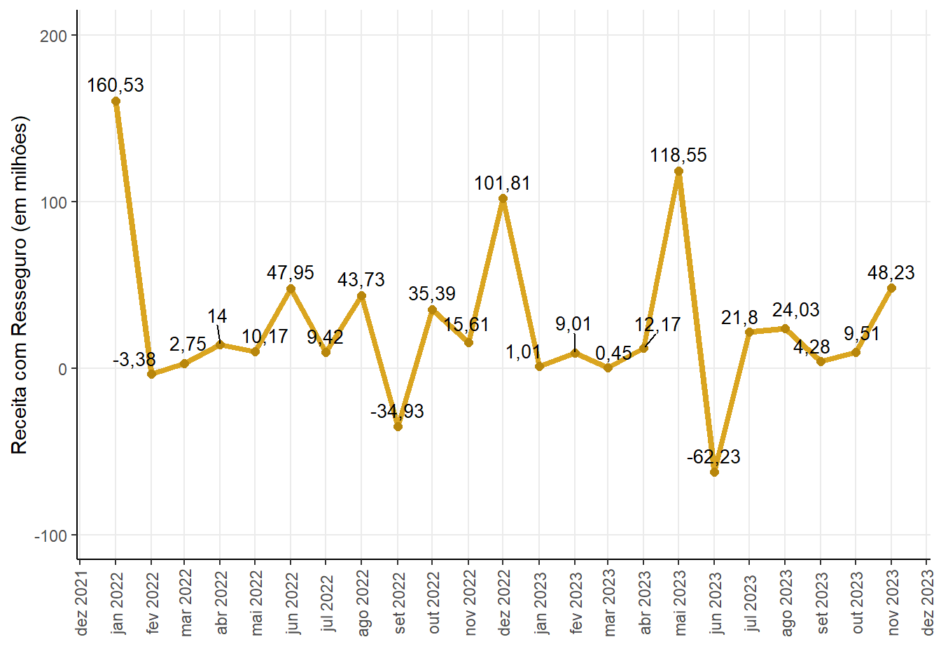
Reinsurance Income (in million)
|
||||
|---|---|---|---|---|
| Min. | Median | Mean | Max. | Std Dev |
| -62,23 | 12,17 | 25,65 | 160,53 | 47,67 |
Historical series of the RVNE for the sector 775 - Insured Guarantee - Public Sector
Current Unissued Risks (RVNE) refers to a situation where the term of an insurance policy has begun, but the policy has not yet been issued.
The Provision for Unearned Premiums - Current and Unissued Risks (PPNG-RVNE) corresponds to an estimated portion of the Provision for Unearned Premiums (PPNG) relating to these risks.
It is important to highlight that the values referring to risks assumed, not in force and not issued are not part of the PPNG-RVNE. In other words, the PPNG-RVNE is specific to risks that are already in force, but whose policy has not yet been issued.
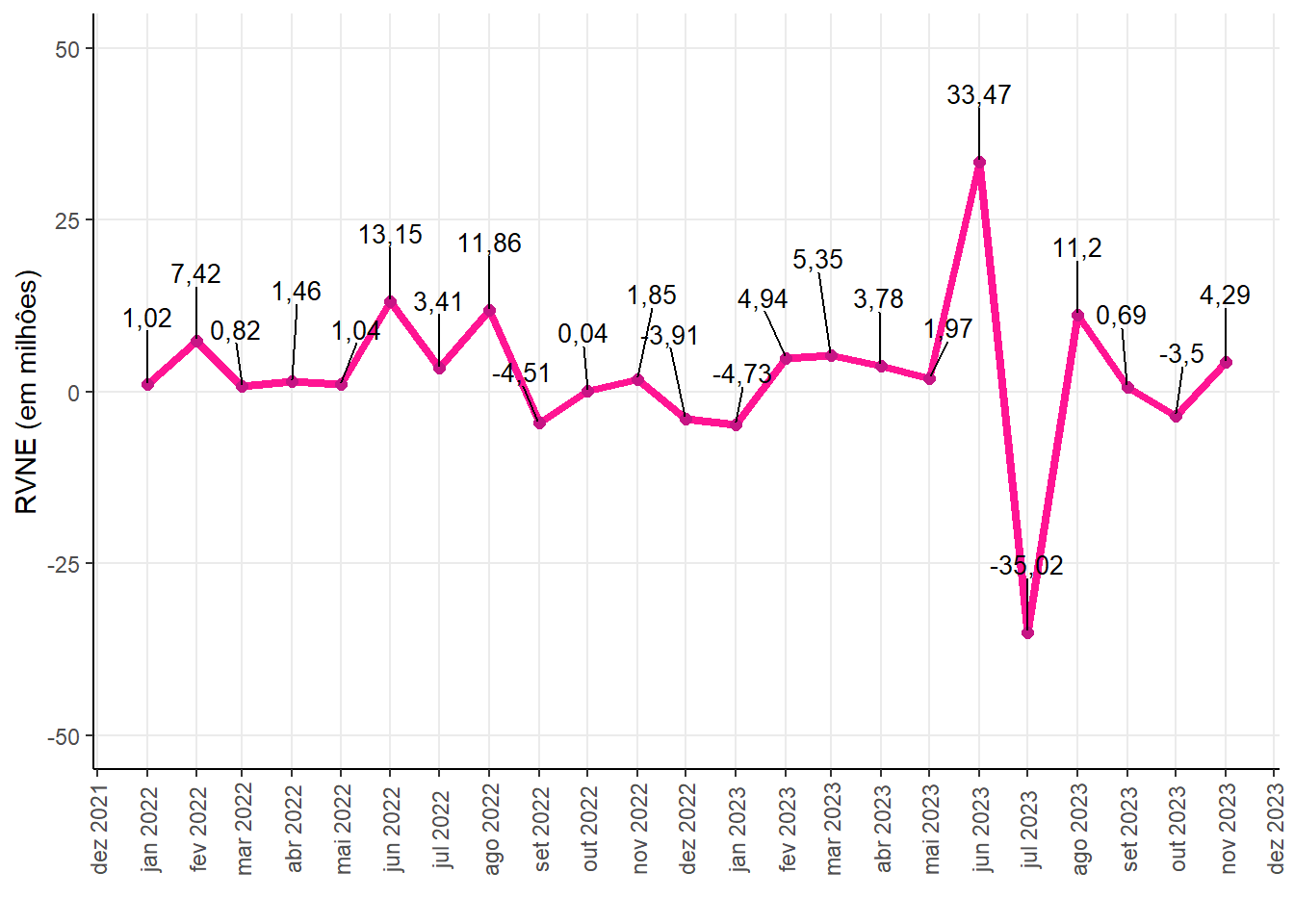
RVNE (in million)
|
||||
|---|---|---|---|---|
| Min. | Median | Mean | Max. | Std Dev |
| -35,02 | 1,85 | 2,44 | 33,47 | 11,45 |
Relationship between variables
In this subtopic we can see the relationship between the variables through the scatterplot and correlation.
The correlation between two numerical vectors is a measure that indicates the degree of linear relationship between these two vectors. In other words, it tells us how much one variable changes in relation to another.
The formula to calculate the correlation between two vectors X and Y is:
\[r = \frac{\sum_{i=1}^{n} (x_i - \bar{x})(y_i - \bar{y})}{\sqrt{\sum_{i=1}^{n} (x_i - \bar{x})^2(y_i - \bar{y})^2}}\]
Where:
- \(n\) is the number of elements in the vectors
- \(x_i\) and \(y_i\) are the elements of vectors \(X\) and \(Y\), respectively
- \(\bar{x}\) and \(\bar{y}\) are the averages of the vectors \(X\) and \(Y\), respectively.
The value of \(r\) ranges from -1 to 1. If \(r\) is 1, there is a perfect positive correlation, which means that as one vector increases, the other also increases. If \(r\) is -1, there is a perfect negative correlation, meaning that as one vector increases, the other decreases. If \(r\) is 0, there is no correlation between the vectors.
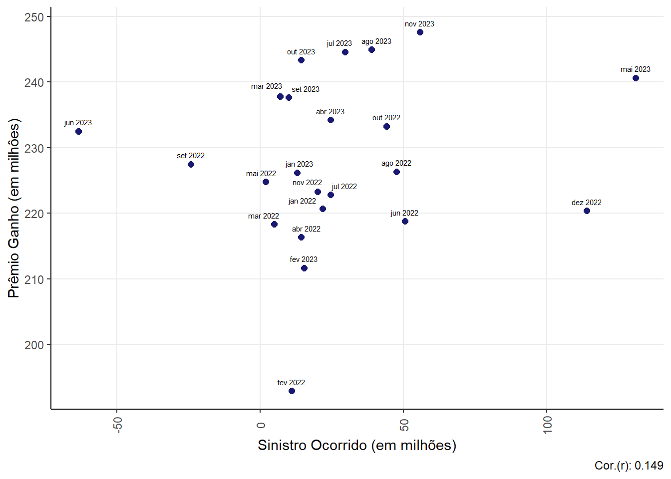
Relationship between Claim (claim ocurred) and Earned Premium
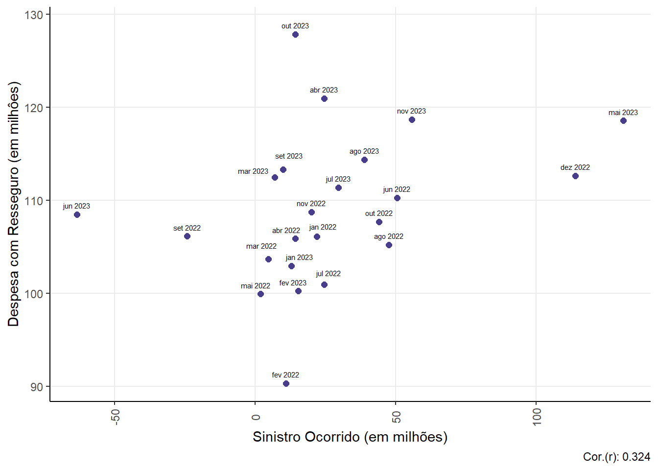
Relationship between Claim (claim ocurred) and Reinsurance Expense
Relationship between Claim (claim ocurred) and Direct Premium
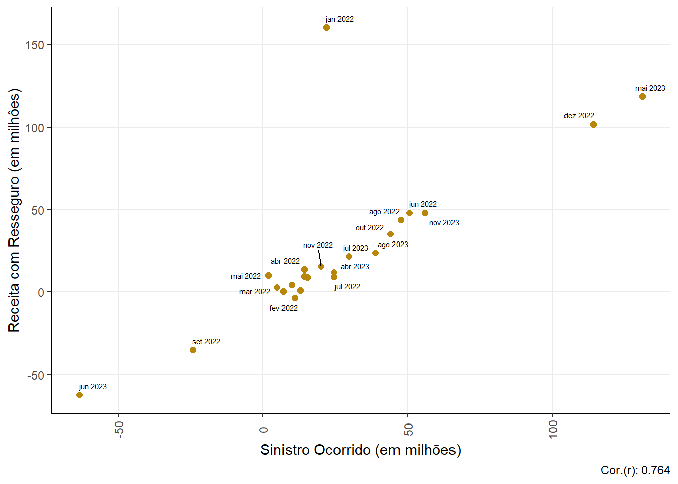
Relationship between Claim (claim ocurred) and Reinsurance Income
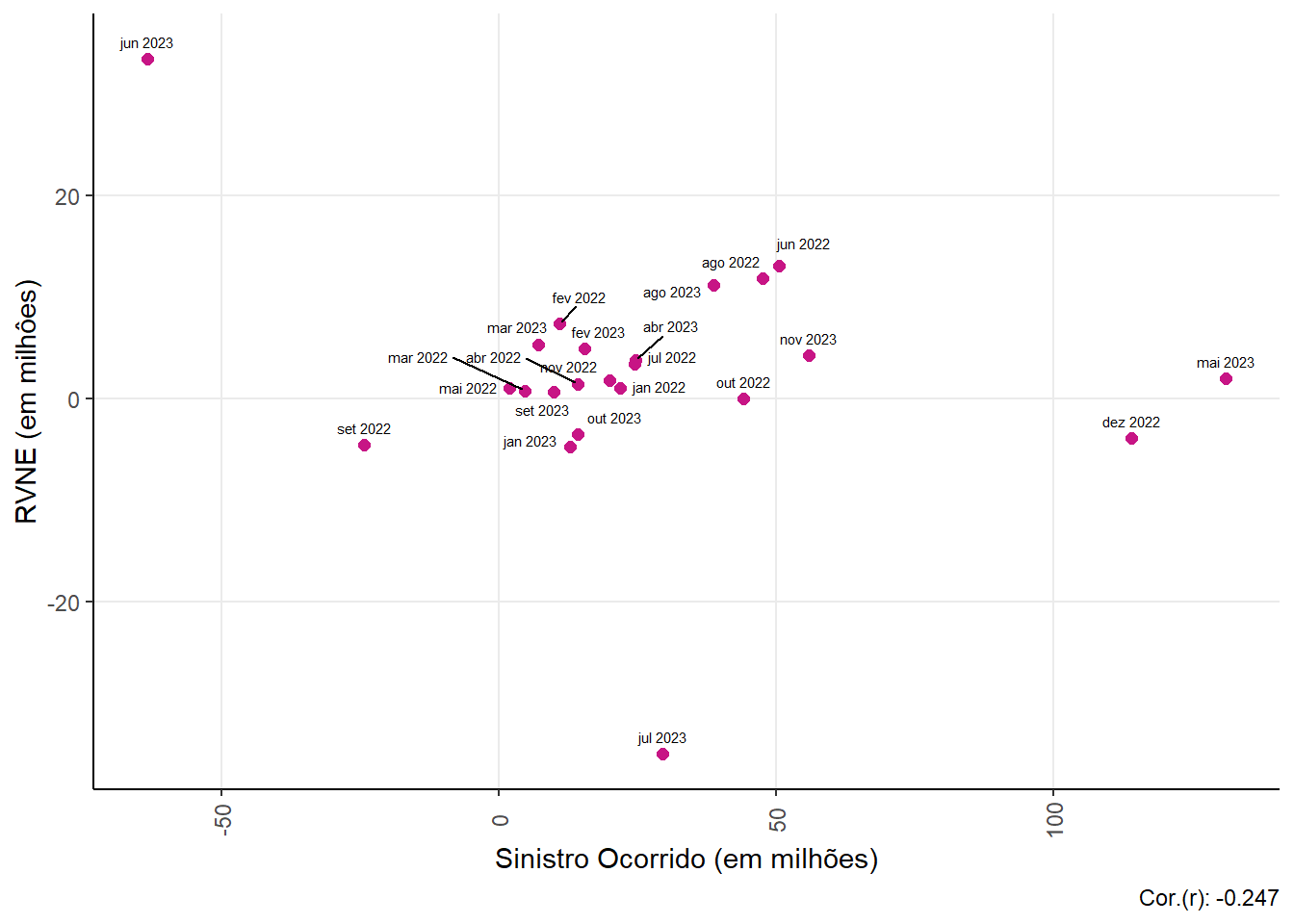
Relationship between Claim (claim ocurred) and RVNE
Statistical model for direct premium prediction
In this subtopic we will begin to build the statistical model for predicting the claim (claim ocurred). We will use strategies to select the covariates that will help us in this estimation and then we will move on to the modeling and validation part.
Covariate selection
Covariates in a statistical model are variables that can influence the response variable we are trying to predict or explain. They are used to control for additional factors that may affect the outcome of an experiment but are not the main points of interest.
Furthermore, they are important tools for improving the accuracy of statistical models, allowing us to control and adjust the effects of secondary variables.
Below we see a correlalogram of the database.
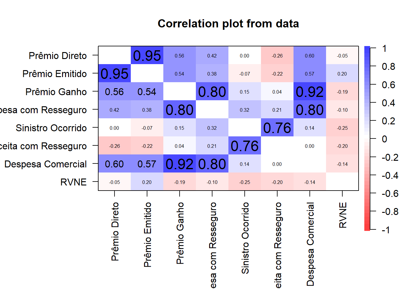
It is noted that some variables have a high correlation with each other, a fact that indicates that we will not need all of them in our model.
To select variables, we will use a multivariate regression model and then apply the stepwise method.
A multivariate regression model is a statistical technique used to understand the relationship between two or more variables. In simple terms, it helps us predict the value of one variable (called the dependent variable) based on the value of two or more other variables (called the independent variables).
For example, suppose you want to predict the price of a house based on its size (in square meters) and its location (city). In this case, house price is the dependent variable and size and location are the independent variables.
The general formula for a multivariate regression model is:
\[Y = \beta_0 + \beta_1X_1 + \beta_2X_2 + ... + \beta_nX_n + \epsilon\]
Where:
- \(Y\) is the dependent variable we are trying to predict or explain.
- \(X_1, X_2, ..., X_n\) are the independent variables we use to predict Y.
- \(\beta_0, \beta_1, ..., \beta_n\) are the regression coefficients that represent the change in the dependent variable \(Y\) for one unit of change in the independent variables.
- \(\epsilon\) is the random error.
Stepwise Method: The stepwise method is a way of selecting which independent variables to include in a multivariate regression model. It starts with an empty model and adds the variable that has the largest significant effect on the dependent variable. It then adds the next variable that provides the greatest improvement to the model, and so on, until adding more variables does not significantly improve the model.
See the values of formula for the multivariate regression model estimated with all variables.
| Characteristic | Beta | 95% CI1 | p-value |
|---|---|---|---|
| Prêmio Direto | 1.6 | 0.73, 2.4 | 0.001 |
| Prêmio Emitido | -1.6 | -2.5, -0.68 | 0.002 |
| Prêmio Ganho | 1.1 | -1.1, 3.3 | 0.3 |
| Despesa com Resseguro | -0.87 | -3.3, 1.5 | 0.4 |
| Receita com Resseguro | 0.87 | 0.61, 1.1 | <0.001 |
| Despesa Comercial | -1.0 | -7.9, 5.8 | 0.8 |
| RVNE | 2.2 | 0.52, 3.9 | 0.014 |
| 1 CI = Confidence Interval | |||
Let’s now look at the values of the model formula after applying the stepwise method.
| Characteristic | Beta | 95% CI1 | p-value |
|---|---|---|---|
| Prêmio Direto | 1.4 | 0.68, 2.0 | <0.001 |
| Prêmio Emitido | -1.3 | -2.0, -0.61 | 0.001 |
| Receita com Resseguro | 0.82 | 0.61, 1.0 | <0.001 |
| RVNE | 1.7 | 0.37, 3.0 | 0.015 |
| 1 CI = Confidence Interval | |||
Therefore, as a criterion for selecting the model variables, we will maintain all the variables that were selected by the stepwise method done above, with the exception of the Issued Premium variable, since it has a high correlation with the direct premium.
Prediction model: ARIMA
As a choice to estimate our model for the claim (claim ocurred) for the Public Guarantee insurance sector (775), we will use the ARIMA model, since the data refers to a time series.
The ARIMA model, which stands for Autoregressive Integrated Moving Average Model, is a statistical model used in time series analysis. Time series are sets of data collected at regular intervals over time. The ARIMA model is used to understand this data or to predict future trends from this data1.
The ARIMA model has three main components:
Autoregression (AR): This component refers to a model that shows a changing variable that regresses on its own lagged values.
\[y_t = c + \phi_1 y_{t-1} + \dots + \phi_p y_{t-p} + \varepsilon_t\]
Integrated (I): This component represents the differentiation of the raw observations to allow the time series to become stationary (i.e., data values are replaced by the difference between the data values and previous values).
Differentiation is applied to make the time series stationary. For example, the first differentiation of a time series \(y_t\) is
\[y'_t = y_t - y_{t-1}\]
Moving Average (MA): This component incorporates the dependence between an observation and a residual error of a moving average model applied to lagged observations.
\[y_t = \mu + \varepsilon_t + \theta_1 \varepsilon_{t-1} + \dots + \theta_q \varepsilon_{t-q}\]
Each component in ARIMA functions as a parameter with standard notation. For ARIMA models, a standard notation would be ARIMA with p, d and q, where integer values replace parameters to indicate the type of ARIMA model used.
As a way of “training” our model, we will use direct premium information from the beginning of 2022 until June 2023. We will then use it to predict the values of subsequent months in order to compare them with the real values.
We will use an ARIMA(p = 0, d = 0, q = 0), where the autoregressive component (p), number of differences (d), and order of the moving average (q) component are 0, which indicates that it is a “white noise” model. In other words, it is a series of errors or residuals that are independent and identically distributed, usually from a normal distribution with mean zero.
To prove these assumptions, let’s check the residuals.
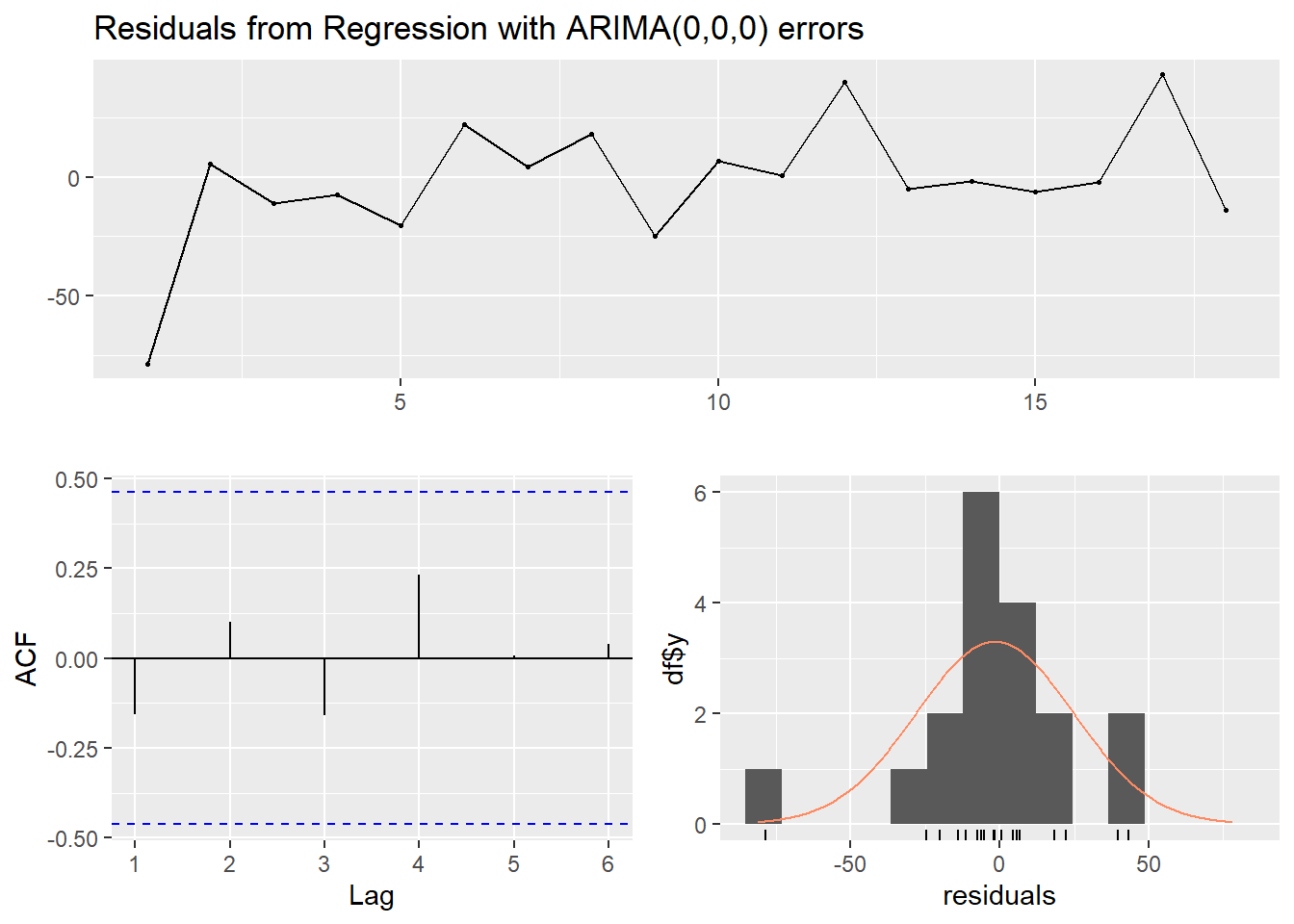
    Ljung-Box test

data:  Residuals from Regression with ARIMA(0,0,0) errors
Q* = 2.7463, df = 4, p-value = 0.6011

Model df: 0.   Total lags used: 4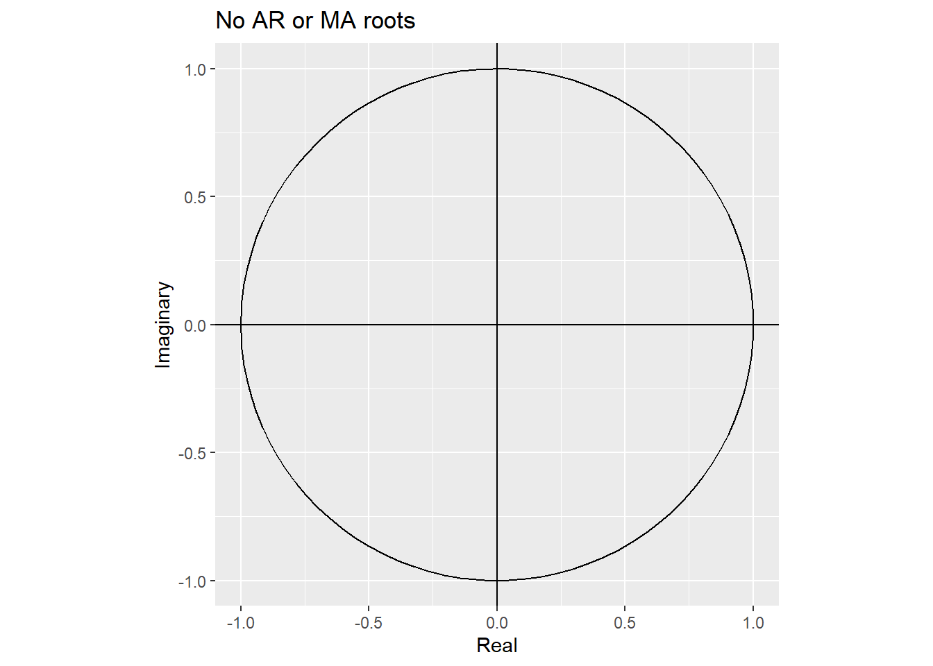
With the Ljung-Box test we can not reject the hypothesis of independence of residues, since the p-value obtained in the test was greater than the 5% significance level.
The acf plot shows that all autocorrelations are within limits.
In relation to the upper graph, we can notice that the residuals (errors) are arranged randomly, which indicates that there is no bias in the model.
Furthermore, the residuals in the last graph are normally distributed. P-value from Shapiro-Wilk Normality Test: 0.04, which indicates that we did not reject the null hypothesis of normality of the residuals, since the indicated p-value is greater than the 5% significance level.
Therefore, let’s look at the estimated ARIMA(0,0,0) model.
| Characteristic | Beta | 95% CI1 |
|---|---|---|
| Prêmio Direto | 0.06 | 0.00, 0.12 |
| Receita com Resseguro | 0.58 | 0.34, 0.81 |
| RVNE | -0.90 | -2.4, 0.58 |
| 1 CI = Confidence Interval | ||
Interpretation of estimators:
Direct Premium (0,06): changing one unit of this variable, there is an increase, on average, of 0,06 million in the claim occurred of the Public Guarantee policyholder sector.
Reinsurance Expense (0,58): changing one unit of this variable, there is an increase, on average, of 0,58 million in the claim occurred of the Public Guarantee insured sector.
RVNE (-0,90): changing one unit of this variable, there is an decrease, on average, of 0.9 million in the claim occurred of the Public Guarantee insured sector.
Below is a table and a linegraph with the estimated values for the months of July to November 2023 with the arima(0,0,0) model.
| Date | Real_value | Point Forecast | Lo 80 | Hi 80 | Lo 95 | Hi 95 |
|---|---|---|---|---|---|---|
| 2023-07-01 | 29,586298 | 62,81 | 26,52 | 99,11 | 7,30 | 118,32 |
| 2023-08-01 | 38,839875 | 26,03 | -10,27 | 62,33 | -29,48 | 81,54 |
| 2023-09-01 | 9,990617 | 31,44 | -4,85 | 67,74 | -24,07 | 86,95 |
| 2023-10-01 | 14,315620 | 26,32 | -9,97 | 62,62 | -29,19 | 81,83 |
| 2023-11-01 | 55,836428 | 41,38 | 5,08 | 77,68 | -14,13 | 96,89 |
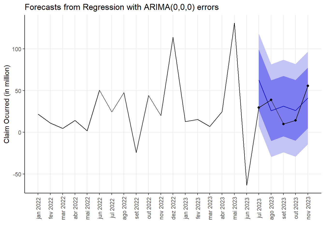
We can note that for the months of July and October 2023 the estimated values were close to the real values (blue line). Furthermore, the predicted values for other month were within the ranges.
Conclusion
In the insurance market, the ARIMA model can be used to predict future trends and patterns. This can help the company prepare financially for these claims and set insurance premiums more accurately. Additionally, the ARIMA model can be used to forecast demand for different types of insurance, which can help insurance companies develop and market their products more effectively.
In the general financial market, the ARIMA model is often used to predict stock prices, exchange rates, interest rates and other financial indicators. These predictions can be extremely valuable for investors and traders as they can help them make more informed investment decisions. Additionally, financial institutions can use the ARIMA model to manage risk and volatility in their portfolios.
In summary, the ARIMA model is a powerful tool that can help companies better understand trends and patterns in their data, make more accurate predictions, and make more informed business decisions. However, like any statistical model, it is important to remember that ARIMA model predictions are based on assumptions and are subject to uncertainty. Therefore, they should be used as one of many tools in a well-informed decision-making approach.
We can mention, for example, our case carried out for the Public Guarantee sector (775) in Brazil, in which the model achieved good adjustments for some cases but was far from adequate for one situation. This distance may be due to the fact that we used little data or even the number of variables used. Maybe I’ll do another study on this soon, thank you very much for reading :).
References
Website:
1library.org: 1library.org. Retrieved from http://www.susep.gov.br/download/menumercado/orientacoes_seguros.pdf (Accessed: February 13, 2024).
Allianz: Allianz Brasil S.A. (2022). Condições Gerais 775 Seguro Residencial. Retrieved from https://www.allianz.com.br/seguros/seu-patrimonio/residencia.html (Accessed: February 13, 2024).
Azos: “Mercado de Seguros.” AZOS. Retrieved from https://www.azos.com.br/ (Accessed: February 13, 2024).
Nubank: Nubank (2023). Prêmio do Seguro: O Que Significa Esse Termo? Retrieved from https://blog.nubank.com.br/vale-vida-nubank/ (Accessed: February 13, 2024).
Doutor Finanças: “Seguros: Teve um Sinistro? Conheça os Seus Direitos e Obrigações.” Doutor Finanças. Retrieved from https://www.doutorfinancas.pt/seguros/seguro-de-acidentes-pessoais-o-que-e-e-como-pode-proteger-nos/ (Accessed: February 13, 2024).
Economia e Negócios: “Por Que os Prêmios Ganhos São Importantes?” Economia e Negócios. Retrieved from https://www.jornaldenegocios.pt/negocios-iniciativas/premio-nacional-de-inovacao/detalhe/pme-desempenham-papel-vital-na-era-da-inovacao-e-dados (Accessed: February 13, 2024).
Forecasting: Principles and Practice. Retrieved from https://otexts.com/fpp2/arima-r.html (Accessed: February 13, 2024).
InfoMoney: “Entenda Como Funciona e Para Que Serve o Resseguro.” InfoMoney. Retrieved from https://www.infomoney.com.br/tudo-sobre/seguros/ (Accessed: February 13, 2024).
Investopedia: Investopedia (2022). Autoregressive Integrated Moving Average (ARIMA). Retrieved from https://www.investopedia.com/terms/a/autoregressive-integrated-moving-average-arima.asp (Accessed: February 13, 2024).
Mutuus: “Resseguro: Entenda Como Funciona.” Mutuus. Retrieved from https://www.mutuus.net/ (Accessed: February 13, 2024).
Mutuus: “Seguros: O Que São e Quais Tipos Existem?” Mutuus. Retrieved from https://www.mutuus.net/ (Accessed: February 13, 2024).
Government Website:
- Superintendência de Seguros Privados (SUSEP) (2023). Prêmios e Sinistros. Retrieved from https://www.gov.br/susep/pt-br (Accessed: February 13, 2024).
Academic Journal:
Chambers, J. M. (1992) Linear models. Chapter 4 of Statistical Models in S eds J. M. Chambers and T. J. Hastie, Wadsworth & Brooks/Cole.
Hyndman, R. J., & Khandakar, Y. (2008). Automatic time series forecasting: The forecast package for R. Journal of Statistical Software, 26(3), 2-7.
Venables, W. N. and Ripley, B. D. (2002) Modern Applied Statistics with S. New York: Springer (4th ed).
Wang, X., Smith, K. A., & Hyndman, R. J. (2006). Characteristic-based clustering for time series data. Data Mining and Knowledge Discovery, 13(3), 335-364.
Wilkinson, G. N. and Rogers, C. E. (1973). Symbolic descriptions of factorial models for analysis of variance. Applied Statistics, 22, 392–399. doi:10.2307/2346786.